What
can we expect from a HF propagation model ?
|
 |
|
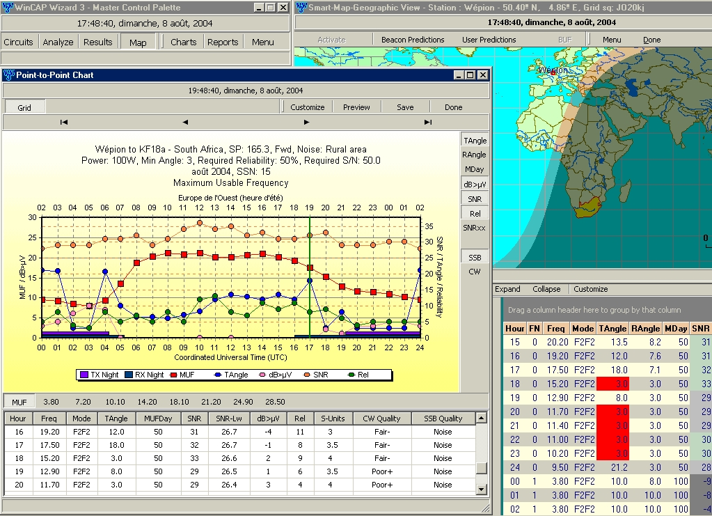
Gray
line map, Results inspectors and Point-to-Point chart created with WinCAP Wizard 3
for a single circuit between ON and ZS. Several parameters are displayed like Takeoff angle, SNR, Reliability,
Signal Strenght, MUF, etc. In this case, with 100 W PEP sent in a vertical antenna, the signal received in ZS
is weak with QRN (S-unit = 3, S/N=31). |
Setting
of a VOACAP model (IV)
To
be complete, here are all parameters (as of the 2004 release) that must be properly set in a propagation
program like WinCAP Wizard 3 using the
VOACAP model, two propagation analysis
tools that are reviewed in the linked pages.
The transmit terminal (TX)
- Transmit power and losses :
use the input power delivered to the antenna less losses in transmission lines or antenna
couplers (e.g. checked on a external SWR-meter).
- Power variation with
frequency : if the power difference exceed a few dB, it can be compensated by
adjusting the antenna gain. In some antenna designs the radiator can be moved
away or bring closer to the parasitic elements. However this change affects also
the F/B and F/S ratios.
- Select the right antenna for each
band : useless if you use a multi-band design. However most advanced programs
take into account several antenna types and apply them to a range of bands. In
addition, with a directional array, don't forget to set the Azimuth field in the
right direction (although you can always work a station using the side or the
rear lobe of a beam !)
- Select the correct S/N ratio
(aka Service type) : SNR gives you a measure of the communication circuit quality;
it defines whether a band is open or closed for a specified reliability level.
Being given that it is an important source of error, it requires some
more explanations.
SNR is a monthly median signal-to-noise
ratio value expressed in dB. It is different in SSB and CW, this latter mode allowing much more noise on
bands and poorer working conditions. This parameter is often split in several
fields : S/N (SNR), S/N reliability (SNR-Rel) and S/N required reliability
(SNRxx). The reliability is the percent of time that the S/N ratio exceeds the
required reliability. The reliability is defined as the fraction of days that
successful communication may be expected at a given date at the specified time
and frequency. It represents thus the expected average performance during
undisturbed days of the month. Based on field experience, this is generally
considered to happen when the geomagnetic index Ap ≤ 27 and the K-index
≤ 4. By default SNR-Rel = 90%, the industry standard. Consequently the required
reliability (SNR-xx) is the S/N ratio exceeded on 90% of the days. However,
amateurs content of a SNR-Rel = 50%.
The
required SNR reliability doesn't appear out of the blue. It depends
on the operation mode bandwidth as follows :
SNR
= 10 + 10 log (bandwidth in Hz)
For
example, a 3 kHz bandwidth SSB signal gives a SNR of 45. A 500 Hz CW
tone is close to 37. It is thus useless to require an SNR higher
than 50%, excepting if you want to work in "Hi-Fi"
conditions or in modes offering a larger bandwidth.
SNR charts are very
instructive once the coverage area from the station has been understood. In a
VOACAP model for example "point-to-point circuit graphs" (a
propagation estimation along two stations including all their properties)
showing the S/NR and SNR-Rel vs. the time and band can be animated through their ranges to better understand when the
bands will be open for a particular circuit.
Now,
a tiebreaker : we know that the VOACAP model can display many
variables. A common question is whether the signal
or the SNR level must be used to measure the circuit quality ?
Intuitively
we have a tendency to check signal predictions, what most freeware or low cost propagation programs used by
default, because most if not all modern receivers have a built-in S-meter, and it is common practice
to compare relative receive signal strenght between stations.
However this value assumes that incoming
signals are transferred to the receiver without any loss.
When the sky wave is reflected by grounds of different dielectric constant and
permeability (land, rock, sea water, etc) or penetrate in a noisy environment, it is far to be the case.
You can also loss more than 50% of power in using a system badly tuned. So, to avoid
taking into account these variations, it is more reliable to use
the signal and noise levels (dB>μV) to calculate SNR predictions because they are
treated as a ratio that remains unchanged by individual station factors.
The receive terminal (RX)
At
the other end of the circuit it is often the big unknown, the terra incognita of
your call. This section is often ignored or amateurs set default
values as it is often difficult to specify the working conditions of a remote
station that sometimes you even don't suspect the existence or the working
conditions !
In
theory here are the parameters to take into account :
- The remote transmitter power
-
The remote antenna specifications (model, gain and bearing)
- The man-made noise level at
the remote site (or at least try to know is he works in the country or in a large
city where QRM is expected to be stronger)
Tips : If you have not the
least information about your remote station, use an isotropic antenna (vertical)
with a 3 to 6 dB gain and select the most appropriate type of area (residential,
rural, etc). But as soon as you work that station, try to get the
specifications of his/her antenna and the type of city in which he or she lives
to improve the forecast.
Here
also if you have not the least information about the remote antenna system, specify an
isotropic antenna with a 3 to 6 dB gain.
Reception Area predictions
Also
named Area coverage, this parameter permits to check if your signal can be heard from
the specified receive location in estimating the noise level at the remote site.
Area coverage
It shows transmission or reception
areas, the latter displaying the result in a chart.
To get an accurate forecast,
and especially to know the Most Reliable propagation Mode
(MRM) it is important to match the antenna radiation pattern to the elevation angle
set in the simulation. In this way you can determine whether
or not your antenna system performs at best
The area coverage
permits to compare the effects of using different antenna
designs (e.g. dipole, vertical, beam, etc). In addition the effect of the
ground can be estimated (signal losses over lands, better propagation over seas, etc).
When
displaying the reception area it is easy to show the gain of an
antenna and see how far goes its radiation pattern (e.g. Yagi vs. vertival).
MUF, LUF and FOT charts
To
answer to our first two questions, when we wonder what band
will be open at what time to reach such a DX country, a
part of the answer can be found in calculating what Maximum Usable Frequency
is generally open 50% of the time; this median value is
called the MUF. Remember that 50% means a 50-50 chance to work in
the specified conditions. That means also that sometimes you will
only have 1% of chance to work that DX, at another occasion 100% of
chance to work it, but in the average 15 days per month the higher
frequency will be open as predicted. It's a good news, but don't go
too fast...
The
MUF is a statistical value associated to a determined degree of
reliability, and thus, it doesn't tell all the story. As all median
value, it gives however a good overview of the range of frequencies
over which we expect some DX openings. But what's the matter below
and above the MUF or using a different reliability ?
We
have first to know that the MUF strongly depends on the ionization level of the F-layer, and
is used to define the uppermost frequency that is reflected by the F-layer at a distance of 3000
km from the transmitter as shows the graph displayed at right.
Frequencies
well below the MUF are affected by the low ionospheric layers at
daytime that have a tendency to lift the Lower Usable Frequency,
aka LUF. The D-layer shows a strong absorption while the E-layer
reflect often shortwaves more than expected. So, on the 40-m band
for example, by 11 AM and 3 PM local time in summertime, we can
experiment deep QSB due to respectively an increasing and decreasing
of the D-layer density and its raising/descent to higher/lower frequency.
This QSB affects transmissions with a fading up to 9 S-point during
some seconds to some tens of seconds repeating during tens of
minutes ! On the contrary, above the MUF your chance to make
contacts are almost null. Due to their high frequency, sky waves are
not more reflected by the F-layers (F2 or F) and escape into space.
Using
sky waves it is thus impossible to work on frequencies too away
below or above the MUF.
 |
 |
|
At
left, a first way to display the MUF. This map was prepared
for 3000 km radio signal paths by the Solar terrestrial dispatch
(spacew) and shows in addition the gray line, the auroral oval and the
sun position. Click on the image to get a real-time update from
DX.QSL.NET.
At right, two other views, more traditional, displaying the MUF and LUF
as a function of time. HFProp
uses either an iso-contour map showing critical
frequencies on the world map for a specified time and circuit
(here from ON to FY) or it displays the MUF and LUF curves in
a chart vs.time.
|
|
The Highest Possible Frequency, HPF, is the
upper usable limit exceeded 10% of the time, or 3 days per month,
or say in other words, in exceptional conditions. During the 90% of
time we should use the Frequency of Optimal Transmission (name after the
French original words), aka FOT. It is defined as the statistical frequency during which the MUF can be exceeded
of 85% (what writes also FOT = 0.85 x MUF). It is thus lower than
the MUF as is reliability is higher. This range of frequencies
spreading between the FOT and the HPF is 4 MHz wide or larger, sometimes so wide
that it includes two ham bands. To know the probability to use such exceptional
conditions, there is only paramater to check : the "required reliability"
of the signal-to-noise ratio (SNRxx or SN-Rel) for the specified circuit.
At last, the MUF predicts ionospheric
conditions but without taking into account other variables (noise, antenna gain,
etc). As it, the MUF chart can thus be misleading and give disappointing
results. It should be used with the SNR predictions to get an accurate measurement
of the circuit quality.
Beacon
predictions
HF beacons from the NCDXF/IARU
international network transmit without interruption in high speed CW
(22 wpm) on various HF frequencies. They can help to "feel" the propagation and see
openings towards each of the 18 countries from which they transmit.
However, used without more
information, the estimation is not very accurate and you need to
take into account additional data like the SSN (smoothed sunspot
number), MUF, required reliability and receive antenna properties to
name some important factors.
Summary
chart
As its title states this chart
provides a general overview of the circuit from one end to another. It was
devised by George Lane, the VOACAP sponsor, at the time he was working with the U.S. Army HF
communications.
This chart is similar to
a MUF chart but includes all system variables so that you can get at a glance the system
integrity at any frequency or time of the day. It is very useful because performance
of your station and your chances for making contacts in good
conditions depend on the correct adjustment of all variables of the system. Therefore
a "good" propagation prediction program, I mean an accurate model and complete
should be able to help you optimize your working conditions and provide you the expected success in DXing.
Next chapter
Running
predictions |