IRIS TURORIAL
Photometry
Introduction: fast photometry starting from the contextual menu
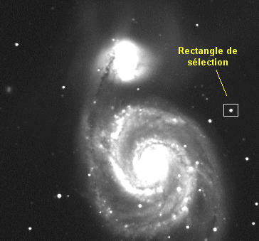
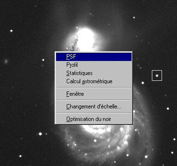
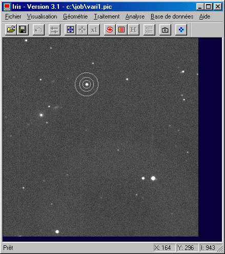
In the image M51 define a small rectangle around a star. For that, drag with the mouse by pushing the left button. The rectangle must be sufficiently large to include all the star signal, but not much larger to avoid including in calculation a significant the background noise. If the shape of the rectangle is not appropriate you can start again the operation:
To call the contextual menu by making a click right in the image. Run the PSF command (PSF = Point Spread Function) :
Iris open a window in which is displayed parameters concerning selected star:

These parameters result from an analysis consisting to modeling of the shape of star by a mathematical function (a two dimensions gauss function). X and Y are the co-ordinates of the center of star in pixels (the origin of the co-ordinates is in the bottom image, on the left and begin with the point (1, 1). Parameter I is the intensity of star. Be carefull, it is not a question of the intensity to the peak of star, but of the sum of the intensity of the pixels forming the star, estimated starting from gaussian modeling (it is thus the volume of the star). The parameter B is the level of the local sky background (in Analog Digital Unit). Finally FWHM X and FWHM Y represent the Full Width At Half Maximum of the star along the X and Y axis respectively.
Click OK. Call the Dispaly data command from the Analysis menu. The window contains same information of PSF dislog box, but in a permanent way.
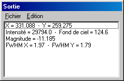
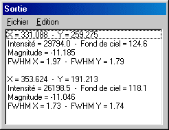
By way of exercise carry out PSF analysis on another star. The contents of the Output window are then updated:
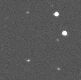
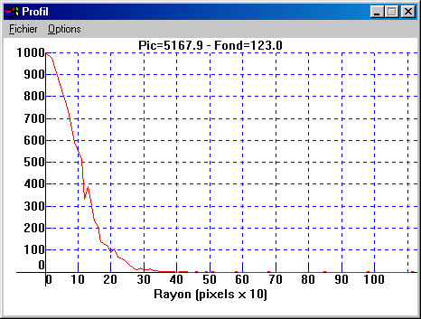
Let us continue the browsing of the contextual menu. After having defined as above a small rectangle around a star (unsaturated, it is significant), run the Profile command. A graph is displayed:
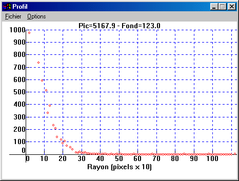
This graph represents the radial photometric profile of the star. The vertical axis is graduated in relative intensity and the horizontal axis represents the distance in pixels relative to the geometrical center of the star. You can check on this graph that the FWHM is well about 2 pixels. One can also notice as the influence zone of the star spread out over at least a radius of 3 pixels.
You can easily modify the aspect of the graph by activating Options menu. For example :
The aperture photometry
We will analyse a sequence having generic name VARI, containing 78 images of the NG C677galaxy field. The images were acquired the 23/11/1998 from 18H45 UT to 22H36 UT. This field contains a detected variable star little time before. The goal of the observation of almost 4 hours is to carry out a light curve of the object. The images were taken in suburbs conditions with a 190-mm flat-fielder (focal length of 760 mm) and an Audine camera. The exposure time is of 120 seconds for each images.
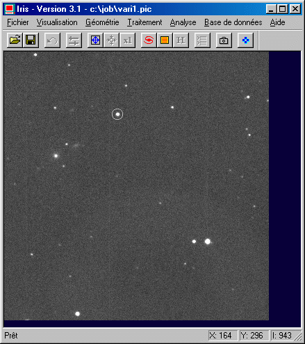
For display the first image of the set (VARI1.PIC):

NGC 677 is located at the cursor coordinates (75, 236). The variable star is at the the coordinates (243, 306).
We saw in introduction a method allowing to calculate the signal recorded in the stellar image by using a Gaussian model fit. The method is powerful, but it can be often put in competition with the technique of aperture photometry. The latter is simpler to implement, more controllable in the situations where the star field is not too dense, and sometimes more flexible to use. The aperture photometry can be employed to carry out high precision measurements.
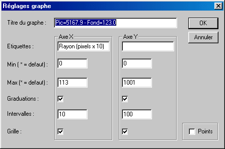
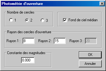
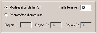
Open the dialog box Aperture photometry of Analysis menu. Enter the following parameters:
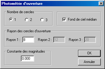
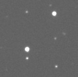
Validate the choices by clicking the OK button. The pointer of mouse changed from an arrow to a circle, of 8 pixels radius in the case present (it is the parameter Radius 1 of the Automatic photometry dialog box).
Center the circle on a star, then click the left button of the mouse:
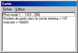
The result is displayed in the output window. The first line gives the type of photometry (only one circle here), then the coordinates of the center of the circle. The second line gives the number of pixels located inside the circle (it is the surface of the circle in pixels). The last line provide the sum of the intensity of all the pixels located inside the circle. This last number includes at the same time the signal of star and signal of the sky. To extract the signal itself from star, it is necessary to take a second measuret by positioning the circle where there are no stars (but if possible in the immediate vicinity of the object measured for exclude major sky non uniformity). Example:
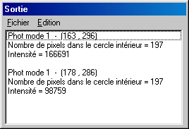
The star signal is thus 166691 - 98759 = 67932 ADU (ADU = Analog Digital Unit).
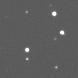
This last result can be obtained in a more expeditious way by selecting the two circles option:
Center the circles on same star and click on the left button of the mouse:

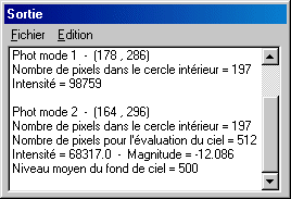
The level of the sky is this time obtained
by summing the signal between the two circles. More precisely, the sky level
is the median of the intensities in the annulus (because the option
Median sky is selected in the Aperture photometry window). Median calculation
is advantageous than a simple average because that makes it possible to
partly eliminate the influence from specific parasitic objects in the annulus
(weak star, cosmic ray, etc). Iris in addition, adds a 3 sigma rejection of
deviants pixelt.
The proper
intensity of star is returned: 68317 ADU, which
is close to the intensity calculated previously. Moreover, the magnitude is
also compute from this intensity (via the formula m = -2,5 X log [intensity]). It is
a relative magnitude because the magnitude constant of the system is not defined,
but the information is very valuable for compare magnitude of stars in
the same field.
It is also possible to select a three circle option:
the returned information is the same one as for the 2 circles option. The difference comes from the sky level calculation, in the area defined by the two outer circle. The intermediate ring is not used. It is a guard zone to make sure that no signal coming from the measured object does polluate the sky estimation.
When the star is badly sampled (FWHM inferior to 2-2.5 pixels) the aperture photometry can become less precise (pixel effect). For recover some precison resample the image on a finer pixel grid. The prefered command for this is ASCALE (not the traditional SCALE function). The ASCALE command, which does not have any parameters, use a special algorithm to increase the scale of the current image by a factor two while preserving the intensity per unit of area. If necessary call several times ASCALE.
Automatic photometry of a sequence
We will automatically estimate the photometry of a variable star by using a sequence of 78 images, named VARI (the generic name). The variable star is compared to a set of reference stars, presumedly stable in time.
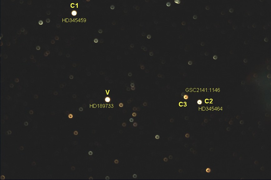
First, from the Analyze menu, run the Select object command. A new mouse pointer appears (four arrows pointer). Click on the first star (#1, it is the variable star). The operationstore in memory the position of the star for latter processing :
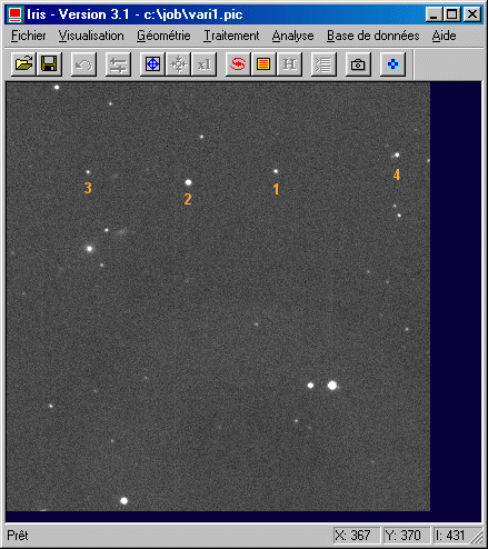
Proceed in the same way for stars #2, #3 and #4, in this order. For stopping the the operation run again Select object command.. You can at this stage start again the selection if necessary.
Open the dialog box Automatic photometry from the Analysis menu:
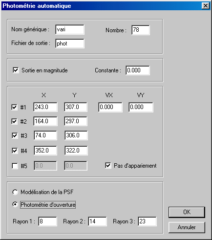
One finds here the coordinates in pixels of four selected stars. It is possible to modify these c-ordinates manually or add a star in the list. The first line always refers to the measured object (here, the variable star).
Indicate the generic name of the sequence to be analyzed. The output file is a text file which contains the result of the photometric analysis. Choose an output in magnitude (if you do not slect the option, the output is in intensity, i.e. in ADU). Select also the option No matching option because one supposes here that the images are aligned through preliminary registration operation.
Lastly, choose the type of photomety: PSF fit or aperture method. Here select Aperture photometry and define the circle sizes.
Click OK for run the calculation. At the end of this calculation, the output window shows the result of the analysis. The first column is the Julian day, the second column is the magnitude of first selected star (the variable object), the third contains the magnitude of second star and so on. All these data are found in the output text file defined by user (here PHOT.LST), for future studies. However Iris create the text file VERIF.DAT automatically in the working dierctory for an immediate control of the good course of operation. It gives the variation in magnitude between studied star and the average of the intensity of the comparison stars. To display the content of VERIF.DAT in the form of graph curve run the Graph command of the View menu (see below an example). Be careful, the file VERIF.DAT cannot be exploited for a scientific analysis.
Photometry of a moving object
The case of the measurement of the magnitude of an asteroid is particular because the object is mobile among the star field. The photometric tool must take into account this movement.
To illustrate the process we will analyze a sequence of 132 images of asteroid 14-SIWA. These images were acquired by Jean Montanné with a 8 inches LX200, the 07/08/2000.
The focal length is of 1016 mm and the pixel size is of 9 X 9 microns (Audine camera). The exposure time per image is 60 seconds. The center of the field is at coordinates AD=21H23m, DEC=-18°23 '.
The acquisition duration of such a sequence can reach several hours, so, drift of the telescope is a classical problem. The automatic photometry function can align the images, but it is generally preferable to use the Stellar registration function of Processing menu. which offers wide possibilities. Alignment on stars of the field is thus a precondition to the photometric analysis and an important step.
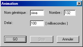
Once registration carried out, a good idea is to examine the sequence by using the animation tool (Animation command of View menu):
The movement of the asteroid is then visible. It is necessary to calculate the displacement in pixels per day. First of all, note the acquisition dates of the first and the last image of the sequence:
> LOAD SIWA1
> INFORMATION
>
LOAD SIWA132
> INFORMATION
Iris
returns the following Julian day:
- for SIWA1: JD = 2451764.3889
- for SIWA132: JD =
2451764.5758
The difference in time is 2451764.5758 - 2451764.3889 =
0.1869 day.
It is now necessary to evaluate the displacement of the asteroids in pixels along the two axes of the images in this lapse of time. PSF tool of the contextual menu is a valuable possibilty for calculate the position of the object in the extreme images and thus to find displacement. An easy way, more quickly, with a high degree of accuracy, consists in adding the first and the last image of the sequence...
|
|
|
|
... then run command DIST from the console. It does not have parameters. Iris invites you to click on two objects of the field for evaluate the distance in pixel which separates them and the projection along the two axis of this distance. Click on the first image of the asteroid, then on the second image of the asteroid (the precise position of the mouse cursor is not very critical because Iris recompute this position relative to the nearest brigth object). One finds:
DX = -71.377 pixels
DY = -34.993 pixels
The daily displacement of the asteroid in pixels is:
VX = -71.377 / 0.1869 = -381.900 pixels/day
VY =
-34.993 / 0.1869 = -187.228 pixels/day
With the Select object tool of Analysis menu, select in first the asteroid, then two comparison stars (for example):
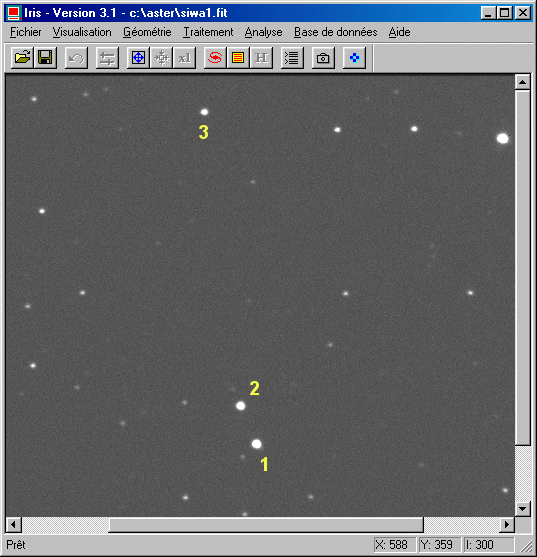
Fill the fields in the following way of the Automatic photometry dialog box:
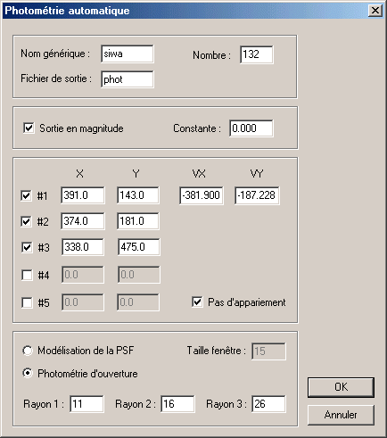
Note be fields VX and VY: the daily displacement is entrer here.
Cliquer on OK. You can see in the output window the real time processing result. Iris produces the result file PHOT.DAT as well the control file VERIF.DAT.
File VERIF.DAT contains whole values which represent the difference in magnitude between first selected star and the magnitude calculated by making the sum of the intensities of comparison stars. The object of this file is to allow a fast control of the result from the Graph function (View menu), but does not have to be used for a scientific exploitation:
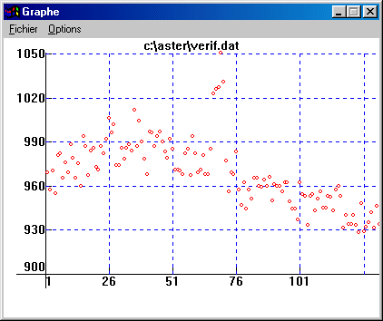
The asteroid curve shows a slow variation caused by rotation on him. The deviating points near the middle of the observation are caused by a star of the field which pollutes measurement.
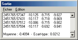
Here an extract of PHOT.DAT file contents:
2451765.41241 -9.906 -9.570 -9.603
2451765.41323 -9.992 -9.535 -9.694
2451765.41404 -9.970 -9.632 -9.700
2451765.41487 -10.053 -9.553 -9.711
2451765.41568 -10.017 -9.574 -9.747
2451765.41650 -10.008 -9.611 -9.628
2451765.41734 -9.929 -9.535 -9.740
2451765.41816 -9.937 -9.501 -9.629
2451765.41898 -9.996 -9.556 -9.646
2451765.41981 -10.019 -9.569 -9.725
2451765.42065 -9.979 -9.628 -9.750
2451765.42147 -9.972 -9.584 -9.588
2451765.42231 -9.869 -9.460 -9.447
2451765.42314 -9.869 -9.452 -9.470
2451765.42396 -9.770 -9.388 -9.444
The first column
contains the day Julien (a line per image), then the following columns are
associated with selected stars. In this example the magnitudes are instrumental
(what explains the negative values). You can have magnitudes closer to reality
by filling the Constant field o the f Magnitude constant dialog
box or the Automatic photometry dialog box (Analysis menu).
The file DELTA.DAT is also produced; Here an extract:
1 -0.433339
2 -0.378491
3
-0.449788
4 -0.334538
5 -0.399466
6 -0.363487
7 -0.465965
8
-0.382446
9 -0.358777
10 -0.382895
DELTA.DAT contains the difference in magnitude between the first column of PHOT.DAT file (in theory the variable object) and the magnitude calculated by making the sum of the intensities of comparison stars. It is by tracing the graph of this file that you will be able to possibly detect the magnitude variation of your object.
File DELTA2.DAT is very similar to file DELTA.DAT, but in the place of the sequence number in the first column one finds the Julian day:
2451765.412407 -0.433339
2451765.413229
-0.378491
2451765.414039 -0.449788
2451765.414873
-0.334538
2451765.415683 -0.399466
2451765.416505
-0.363487
2451765.417338 -0.465965
2451765.418160
-0.382446
To check the
consistency of your analysis one should not hesitate to calculate the difference
of the comparison stars find magnitudes. If the first selected star is a
nonvariable star, you can record in particular the level of precision of the
photometric reduction (deviation value returned in the output windows at the
end of the calculation). Here an example:
A good practice to take is to test the photometric precision (standard deviation) by adjusting some parameters, and in particular as regards photometry aperture, the size of circles (in particular the interior circle). Attention also with the undersampled stellar images, which is one of the major factors affecting the precision. Not hesitate to use the ASCALE command. Command ASCALE2 cammand can process a set of images. For example:
>ASCALE2 SIWA I 132
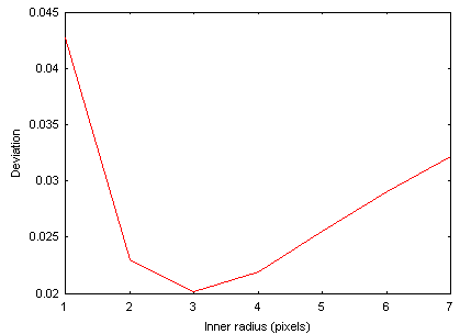
In the example below one traced the value of the standard deviation according to the interior circle radius. A marked minimum is well noted. The corresponding radius is adopted for the present photometric analysis for ultimate result :
Automatic photometry can be carried out by modeling the PSF (PSF = function of spreading out of star):
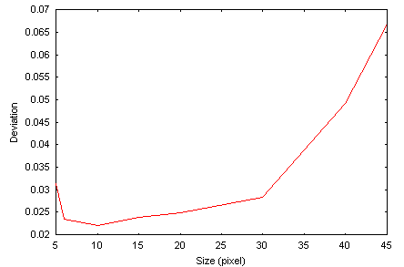
In this case you must specify the size in pixel of the square inside whose the star adjustment is carried out. Just like for the dimension of the aperture photometry circles, you must define this parameter carefully by tracing the standard deviation according its value on a test star. Generally the size of the window is 4 to 5 times the value of the FWHM. If dimension is too large, the software will try to adjust the noise of the sky background, which is not excellent. If the size is too small, mathematical modeling only use a fraction of the star signal, which is not good either. The example below show the photometric error (at 1-sigma level) according to the size of the computation window sziet (for information, the FWHM of stars is here of 2.3 pixels):
Generally, one will prefer the PSF method in the case of the study of a mobile object or when the stars density is significant (blended field), because the size of the analysis zone is smaller than what is necessary in aperture photometry. However, contrary to a generally accepted idea, the ultimate precision in photometry is reached by the use of simple aperture circles. The conjunction of a clean calculation of the sky level (median value plus rejection scheme), of an optimal sampling of the image (ASCALE and ASCALE2 commands, see Mighell, K J & Rich, R. M. 1995, AJ, 110, 1649) and of an optimal choice of for the circle radius based on an least square error analysis, permit to reach ultimate performance with the aperture photometry method. The aperture photemetry is also less sensitive to the deformations of stars caused by guiding error from image to image, a great advantage with the amateur instruments.
The graph below shows the photometric error for different methods on a sequence from 200 images (FWHM of stars of 2.3 pixels). These curves result directly from files DELTA.DAT produced by Iris.
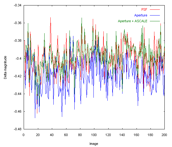
Here the noise in magnitude (1-sigma) statement in these various tests:
Mathematical fit of the PSF: 0.0187
Aperture
photometry: 0.0184
Aperture photometry with a pixels grid twice finer
(APHOT2): 0.0164
To note that for much, the residue of fluctuation is induced by atmospheric scintillation. Only techniques for reduce this is to use a larger telescope or average of contiguous measurements (but at the detriment of the temporal resolution).
Photometry and digital SLR
A
key technique: defocus the image for increase precison et dynamic of the measure...
How to modify the acquisition date of an image
The date is a fundamental parameter for photometric analysis. It is always possible to correct it or to even establish it in an image file.
Load the image in memory:
>LOAD IMAGE
Modify the date by using the SET_DATE command. For example:
>SET_DATE 13/12/2005
for the December 13, 2005.
Modify the hour by using the SET_HOUR command. For example:
>SET_HOUR 16:49:20.3
To check the modification use the INFO command.
Save the image with the updated header:
>SAVE IMAGE
Command INIT_DATE modify the date of a set of images. The parameter of this command is a file descriptor having the .lst extension, which associates an image name with a date and an hour. For example, if the contents of file FILE.LST is (it must have obligatorily three columns):
var1 13/12/2005 16:49:20.3
var2 13/12/2005
16:52:39.8
var3 13/12/2005 16:55:00.4
and if you run
>INIT_DATE FILE
Iris load the image var1 and attribute the date December 13, 2005 at 16 hours 49 minutes 20.3 second. The image file var1 is automatically saved with the new header value. Iris process in the same way the images var2, var3...