Deep-sky image projection into galactic system.
New features
of versions 5.51
Version 5.51 - June 16, 2005
Deep-sky
image projection into galactic system.
Correction of lateral chromatism of photographic lens.
Version 5.50 - June 10, 2007
New features :
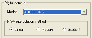
- Possibility to decode RAW file in format ADOBE DNG. Select the option from the camera settings dialog box:
- New HDR processing function.
- Coordinate
projections of stellar images.
HIGH DYNAMIC IMAGERY
New command
REDUCE_HDR3 [GAMMA] [COLOR] [SMOOTHNESS]
REDUCE_HDR3 modifies tone reproduction of High Dynamic Range images. The object is to mapping high dynamic range to low dynamic range compatible with computer screen or photographic print. Compared to commands REDUCE_HDR1 and REDUCE_HDR2, which deal with the same problem, REDUCE_HDR3 offers a better control of coloured contrast. The parameter GAMMA fixes the intensity contrast. The typical adopter value ranges between 1.2 and 3.0. The COLOR parameter fix simultaneously the saturation of the image. The characteristic value of this parameter lies between 0.5 and 3 (saturation increases when the value increase). Lastly, the parameter SMOOTHNESS adjusts a high-pass filter which applies to improve the sharpening. A value should be chosen between 0 and 1 (when the parameter SMOOTHNESS is zero, there is no sharpening is applied).
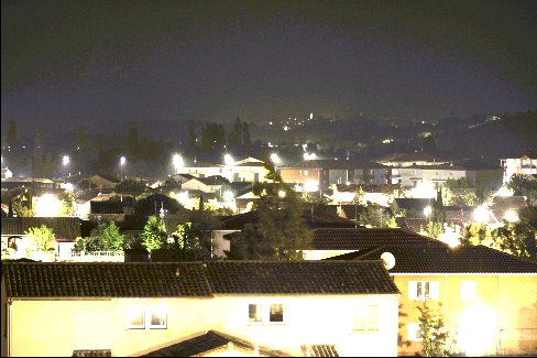
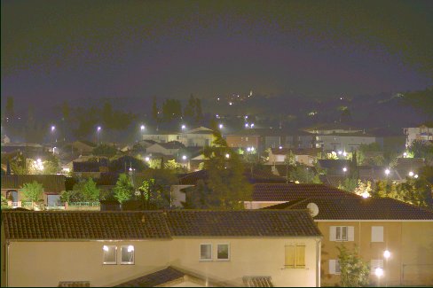
The image below is a typical HDR document. This night city view was carried out with a Canon EOS 400D. It is the fusion of 10 images exposure between 1/60 S at 8 seconds (nearly 3 orders of intensity magnitude). The 10 images were gathered with command MERGE_HDR. Here the final image is displayed using a linear scaling :
The maximum level noted in the images
(street lamps) is 32767. Visualization used here is >VISU 32767
0.
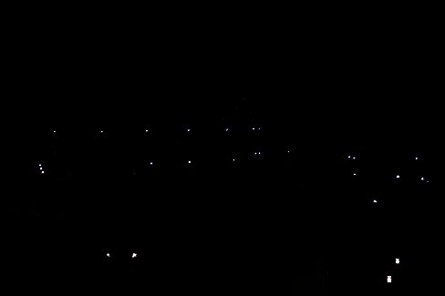
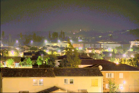
The same image, but displayed for enhance faint part, in a linear intensity scale:
Visualization
adopted is VISU 30 0, which reveals the faints details of the image. But at the same time other parts of the image
are completely saturated (frontages of house, lamps).
The test image after the application of command REDUCE_HDR1:
>REDUCE_HDR1 3.0
The result of command REDUCE_HDR2:
>
REDUCE_HDR2 1.4 0.4
And the result of new command REDUCE_HDR3:
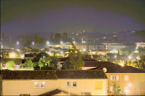
>
REDUCE_HDR3 1.6 0.8 0.5
The image processed with REDUCE_HDR3 shows a good restitution of colors and presents less atefact around bright objects.
MAPPING THE SKY
Iris V5.50 introduces a new set of tools for precise superposition of images of the sky taken with different instruments or at different times or, for assemble images connected perfectly in order to constitute big panorama. These tools are help to manage images capured with wide-angle lens. It is for example possible to build a global all-sky images from a series of elementary pictures. The superposition of the images with the astrometric precision open the possibility of automatic search of new variable stars, comets, etc.
The steps of the operation are:
1 - Search of distortion law of the lens. The step is mandatory for wide-field imagery since one uses optical focal length lower than 135 mm (to fix the ideas). The distortion parameters, estimated once, are a constant of the instrumentation.
2 - Correction of the optical distortion in each image which one wants to assemble by using the parameters found at the preceding step.
3 - Astrometric reduction of the individual images. This amounts associate celestial coordinates (right ascension and declinaison) with each pixel.
4 - Projection of each image in a common celestial map. Map projection is a transformation that convert celestial sphere coordinate on a flat map. Iris proposes up to 7 distinct projections.
5 - The fusion of all the images projected in the same cartographic reference frame into an unique image.
The final result having an astrometric quality, it is for example possible to identify object by their celestial coordinates (right ascension and declinaison).
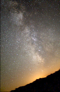
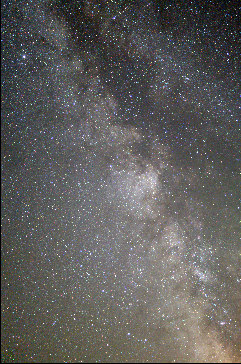
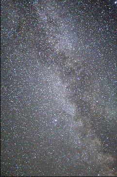
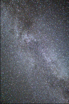
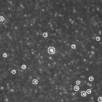
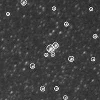
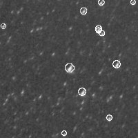
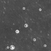
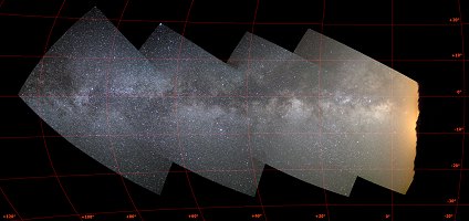
In order to illustrate this procedure, we will process a concrete example of images. Those were acquired by Valerie Desnoux from the Pic-Du-Midi (french Pyr�n�es) with a Nikon zoom used at focal of 18 mm. The camera is a Nikon D70. We have 4 images covering a part of northern Milky Way. Here these 4 images in very reduced version (the original documents have a size of 2014x3039 pixels):
|
|
|
|
|
STEP 1: EVALUATION OF LENS DISTORTION
In absence of optical distortion, the linear distance R between the center of the image and the position of a star is related to the angular distance a of this star compared to the optical axis through the formula:

were F is the focal length of the lens.
This relation indicates that in the case of the use of a perfect optics, the image can be seen like the projection of the objects on a plane tangent to the celestial sphere at the level of images centers. It is a projection known as gnonomic.
In presence of optical distortion the tangent foumula is not valid any more. To find distortion parameters we compare the actual stars position to the position in the absence of distortion. Let us choose for that image FIELD3 (image FIELD1 for example is not convenient because a significant part is out of the star field).
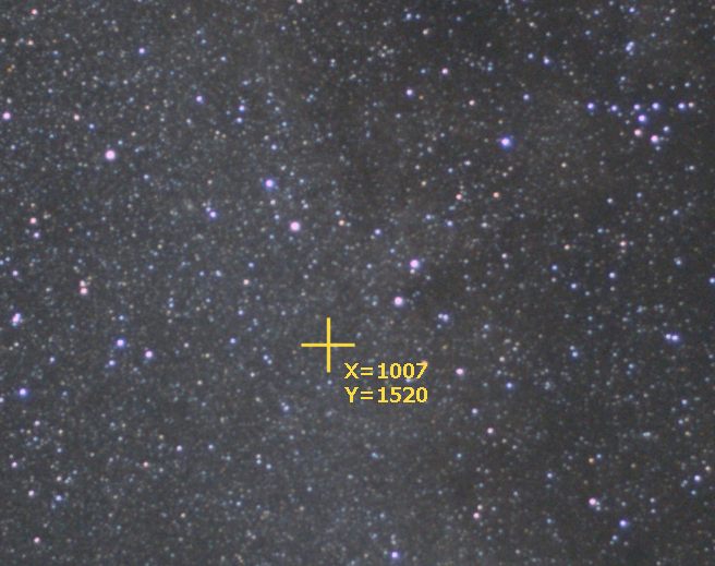
From a sky atlas locate the approximate equatorial coordinates of the image center (dimension of the image is 2014x3039 pixels, from where coordinates of the center is (1007, 1520)). Below, the central part of FILED3 image (attention, it is strongly recommended to direct the noth up of the image, use for that the commands MIRRORX, MIRRORY, MIRRORXY):
A digital card of the sky can help for find the coordinates, here delivered by Megastar software:
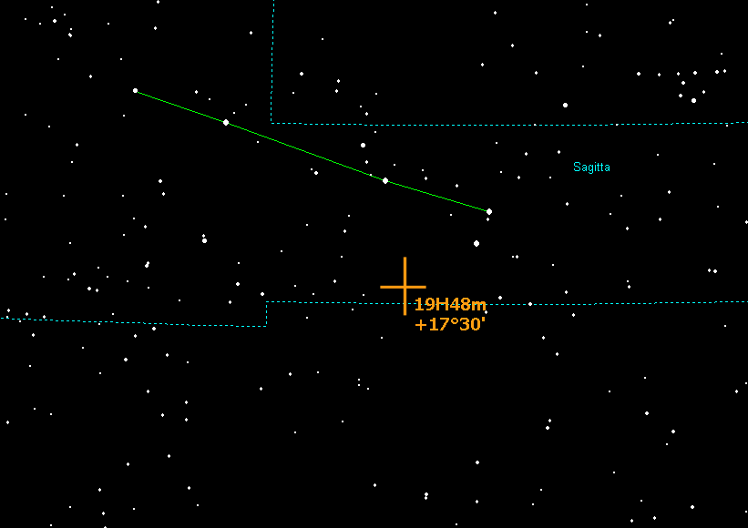
The required equatorial coordinates are: RA (right ascension): 19h48m, DEC (declinaison): +17�30 '. A high degree of accuracy is not necessary (error of few minutes for angular values do not affect the result of calculations to follow).
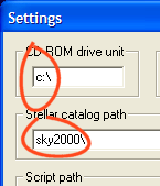
The goal is now to superpose a synthetic map (extracted for a star catalog) to the real image. SKY2000 catalog is ideal for us because it contains all stars more brilliant than magnitude 8 at least, which is largely sufficient to calibrate images acquired until the focal length of 135 mm (and digital DSLR). The SKY2000 is compact and contain stars up to magnitude 9. Download the SKY2000 catalogue here (6.8 Mb). Decompress the zip file in a directory of your hard disk, for example C:\SKY2000:

Now call Settings... dialog box, File menu, and precise the directory containing your star catalogue:
Run the command Display a sky map... of Data base menu:
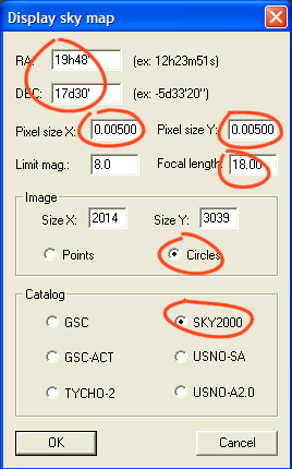
Enter equatorial coordinates of the image center (item RA and DEC). It is also necessary to provide the size of the pixels of the detector in millimeters. For the Nikon D70 camera we adopt a size of pixel of 0,005 mm (5 microns). The focal length of the lens (or telescope) is also required (here f=18 mm). Select SKY2000 catalog, then finally, select Circles option. In this manner the stars in the card are drawn as small circles (the diameter is proportional to the magnitude), which proves more readable than a traditional map displaying stars in the form of points.
Click OK. At the end of a few seconds the numerical card of the sky is currently displayed on the photographic image in memory (image FIELD3):
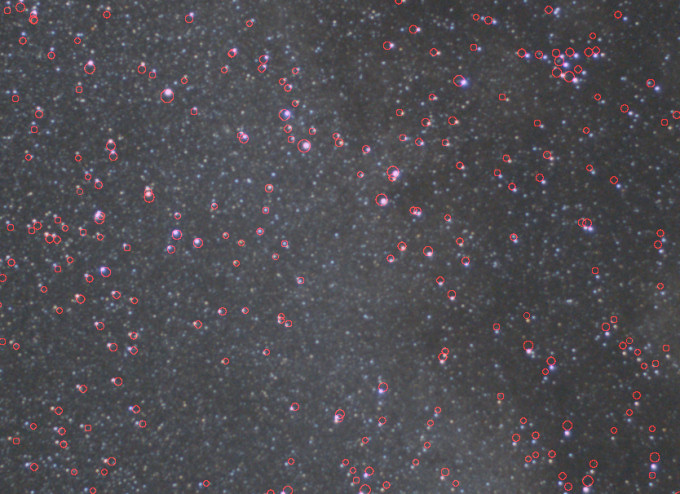
The central
part of image FIELD3 with, in red, the position of the stars extracted from
the SKY2000.
The circles are superimposed on stars for the center of the image. This indicates that the coordinates of the center of the image are correctly evaluated. It appears obvious however with the examination of the result that a field rotation affect the image (rotational angle between the observed image and synthetic map). The centre of rotation is in the vicinity of the image center, which is normal since we have already pre-center the map at this place. The problem is traditional: even if the digital camera is fixed on an equatorial mounting, (orthogonality problem of camera relative to the mount, or polar alignement error, can easily explains the noted rotation). We will seek the value of the angular rotation interactively.
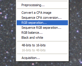
Note: it is possible to exploit images colors, but for efficiency a good idea at this stage of the optical distortion evaluation it is preferable to isolate only a black and white component of the true colors image. The ideal is to choose the green layer (best signal to noise ratio). With the image to be treated in memory, run the command RGB separation... of Digital photo menu:
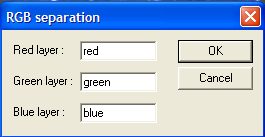
The function produces three new files images in the working directory, corresponding to the components red, green and blue channel of the color image. For example give the names " red ", " green " and " blue ":
Now, load the green image:
>LOAD GREEN
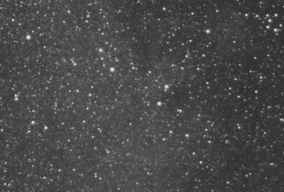
Central part of
the "green" component.
Now a sky map without the real image, but of the same format, is produced. From the command console, enter:
> FILL 0
The image currently in memory is filled of zero. It appears black. Then, open the dialog box Display a sky map... (Data base menu) and cliquer OK without anything change (the preceding settings are preserved). Here a part of the produced map:
Save the image on the disk. Choise "mark" for the file name, for example :
> SAVE MARK
Produce a last image which will be useful for us in little time. Erase the in memory image:
> FILL 0
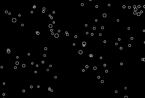
then recall the digital map dialog box, but this times select the Points option instead of the Cercles option:
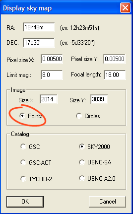
The synthetic stars appear in a stellar form:
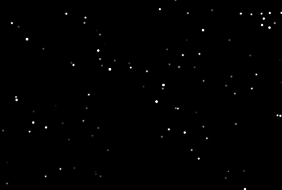
Give the name "reference" to the image on the disk (for example):
> SAVE REFERENCE
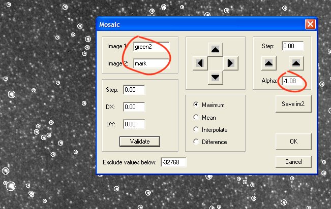
Now run the Mosaic... tools from Geometry menu. We will superimpose the image of the star field (image " green") with the synthetic stellar map " mark". To see the result, click the Validate button. In the representation hereafter, we show the upper left corner of the image:
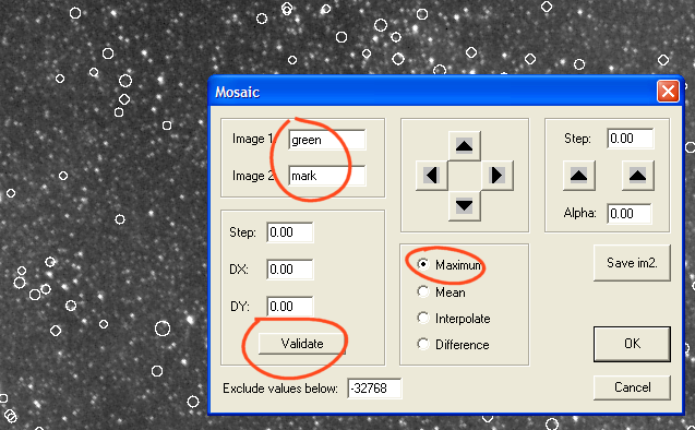
The angular shift between the photographic image and the card map quite obvious. It is even amplified if we examine the corners of the image. We now rotate the digital map relative to its center (try some angular values):
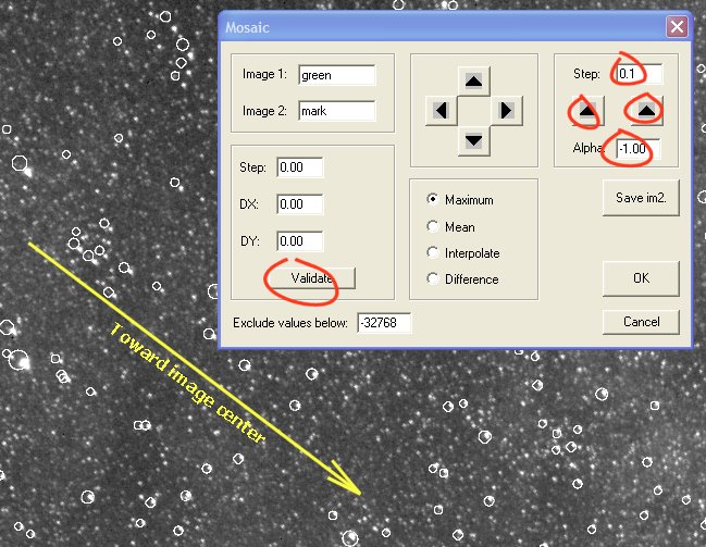
One notes that the card is aligned radially for a rotational angle close to -1.0 degree. Along the radius direction (relative to the image center), the two images are not registered. The principal cause of this variation is the optical distortion. Another possible reason could be a bad choice for the size of the pixels or focal length (what returns to same). It is not the case here because, if one notes that the circles are outside real stars in edge of field, that is reversed while going towards the center of the image. It is the information that "in average" the adopted optical length focal distance (and pixels size) is correct. If the card and the image deviate too radially it is necessary to modify the size of the pixels or the focal length (let us say of 5%) during the synthesis of a new sky map, and test the registration with the image by using the Mosaic.. tool. If need be, to carry out several tests to arrive at the good focal length (often, the focal length indicated for a photographic lense, especially with zoom, is only approximate!).
If the superposition is not satisfactory for the center of the image, you can in addition to the rotation shift along X and Y axis the sky map ( DX and DY values, and remember to give a value for step item).
Note: if the visualization of the image does not appear correct to you when Mosaic dialog is open, it is always possible to modify the visualization thresholds in the course of operation.
Click Cancel because the use of the Mosaic tool that we have just made if only for expose a method allowing to evaluate the field rotation. The image is not corrected physically for the moment. We find -1.0� here.
Run the command Evaluate distortion from stellar image... of menu Analysis:
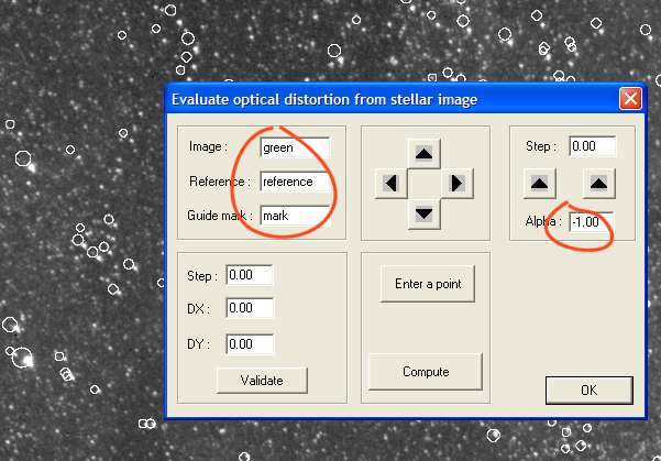
The aspect the dialog box ressembles to the Mosaic tool. It is however necessary to provide the name of three images:
- the image used for estimate distortion (here the
"green" layer of our image color).
- a reference image, containing
no distorded position of stars (here the image "reference" extracted
from the SKY2000).
- an localization image (optional), which shows easily
star positions of the reference image (here the image " mark").
Our goal is to indicate in a selection box many couples distributed in the image including a star of the photographic image and the corresponding star in the reference map.
With the mouse pointer (right button and drag) define a selection box "around" a couples (a synthetic star and a real star). To pay attention to include in the rectangle only the components of one couple (if needed, re-run the selection). Then, click the button Enter a point:
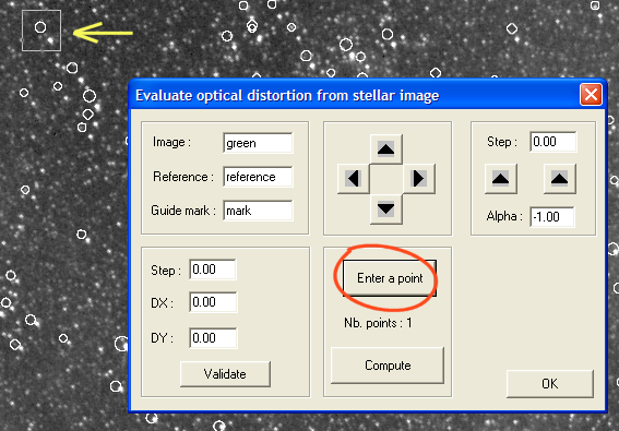
The software has just recorded position of the couple in memory. Start again the same operation for another couple, and so on. Thus record a few tens of couples, distributed well in the image: not forget the corners of the image, the center and intermediate areas:
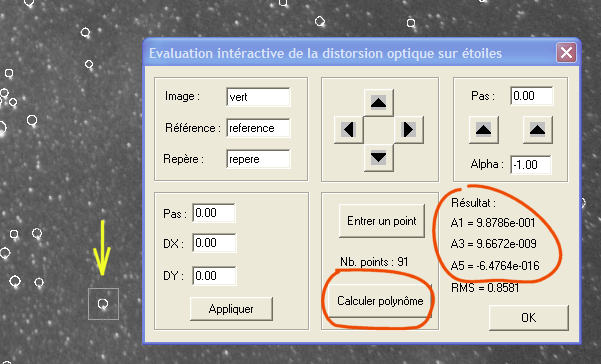
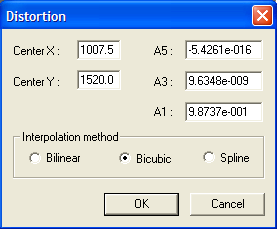
At any moment you can click the button Compute. The coefficients of a polynomial of the fifth degree is returned. The polynome parameters describe the distorsion of the optic. The software return also RMS error of the evaluation (in pixel). The form of calculated equation is:
R is the distance to the center of a point in the corrected image and R' is the position of the same point in the starting image (affected by the distortion). In our example, the fact that the linear coefficient A1 have a close value unit (0,988) shows that we were mistaken little on the actual value in the focal length (and of the size of the pixels too).
To complete the operation close the dialog box (button OK).
The following operation consists in modifying the image geometrically for correct effectively the optical distortion. Run the command Correct distortion... from Geometry menu. You can note that Iris copy for you the value of the coefficients A1, A2 and A3 in the corresponding fields. You do not have to enter the values in theory. Cliquez simply on OK :
Save the transformed image on your disk. For example
>SAVE GREEN2
To check the success of the operation, open the Mosaic tool (Geometry menu), and compare the synthetic image of the sky with the corrected image for the distortion. The field rotation can be also easier appreciated now:
The severe optical distorsion of lens is very effectively corrected: the circles surround stars well now. For better analysis you can explore the 4 corners of the image:
|
|
|
|
|
|
You now let us correct the distortion in the coor image FIELD3. Load this image in memory:
> LOAD FIELD3
Run the command Correct distortion... (Geometry menu). Do not modify parameters, click simply OK. Save the result, for example under name IMG3:
> SAVE IMG3
A significant stage on the road of panorama construction was accomplished. All images acquired with the same configuration optics can be corrected with the same set of coefficients A1, A2, A3. Including for images non astronomical images of course, the distortion default can be now reduced with a very high degree of accuracy.
Recommendation: to lose a minimum of spatial resolution choose the option Bicubic or Spline in dialog box Correct distortion... Calculations are longer, but the restored image is finer.