New features of version 5.30
Version 5.30 - March 4, 2006
You can now define a directory for store your script files (see RUN command). It is necessary to open the Setup dialog of File menu, then to fill field "Script path" with the path of a valid directory:
If the field is empty, Iris search scripts in the working directory.
Use fisheye optics
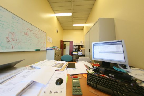
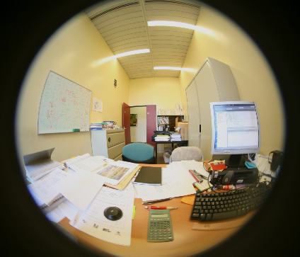
Here a typical fisheye image:
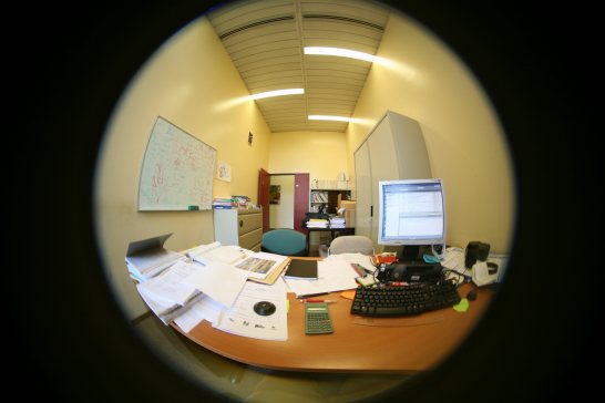
Canon
EOS 5D and Peleng 8 mm f/3.5 fisheye image. The Peleng is a low cost objective but also
a good true
180° fisheye.
The full frame of the EOS 5D is presented in this reduction.
Click here for details about this lens.
Iris V5.30 introduce a new set of geometrical correction commands (Geometry menu):
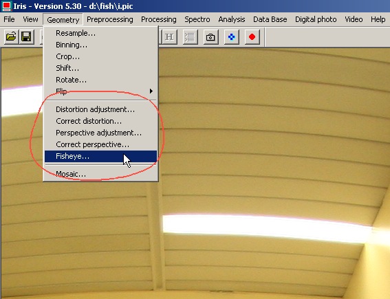
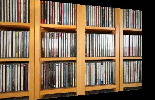
Run the Fisheye... command:
Enter the coordinates of the field-center of the fisheye image. Here x=2200, y=1456. Enter the focal length of the fisheye. Try some values for minimize distortion (if you work on a reduced image, multiply the focal length by the reducing factor). Choose the Bilinear interpolation method for the fast result. Select also the Rectangular projection. Click OK. The spherical fisheye image is now projected on a front tangent plane:
|
|
|
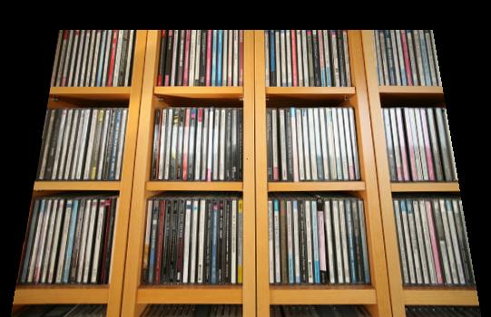
Reload the fisheye image and select a smaller scale factor:
Scale
factor x0.7
You can also adjust the size of the output support. For example:
Output
image of 6000 x 3500 pixels (reduced version).
For the final output, select the Bicubic option. It is a high quality interpolator, that preserve finest details of your image.
The computation time is also reasonnable for big images. The Spline interpolation is the better algorithm but it is very time consuming and the difference compared to Bicubic method is not very significant in the major of situations. Use Spline option only for a very final touch or for process small images.
Consider now this all sky view (the lens is oriented toward the zenith, taken from my personal suburb observatory):
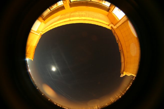
Canon
EOS 5D + Peleng 8 mm fisheye. From my balcony observatory.
Select the Panorama option and the following parameters:
The next figure give the signification of the parameters:
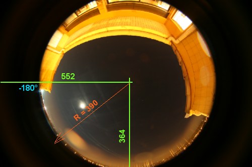
The Angle parameter define the position angle origin of the future panoramic view. The Deg./pixel parameter is the horizontal scale of the panoramic view in degree per pixel. The result:
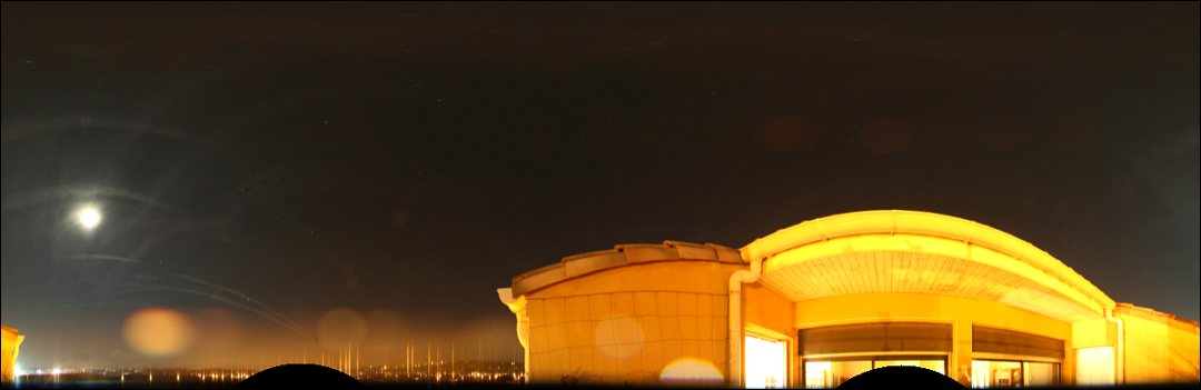
The
panoramic image.
The
position angle is now -80°.
For obtain the same result from console commands, enter:
>LOAD FISHEYE_VIEW
>REC2POL2 552
364 390 -80 0.3
>MIRRORXY
>MIRRORX
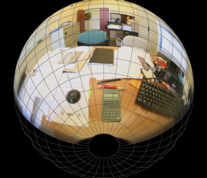
Try now the Sphere projection (remember to reload the original fisheye image before).
|
|
|
After projection, the scene is as if you see in reflection on a sphere.
Edit the text below (use WordPad application for example):
0
0 90 0
848 727
424
364 370
0 0
-180 180 -90 90
0 0
0 1
10 10 3
and save with the name SPHERE.LST (for example, only the extension .LST is important). It is a parameters list for the MAP familly commands. For simplification reason, use the working directory. The signification of the given parameters is:
For a full description of the MAP capability click here. For some application examples, click here.
With the assistance of the mouse pointer measure carefully that the center of the spherical image is located at the coordinates X=424 and Y=364 (you can enter fractional values). Another significant value here is the radius of the sphere in pixel (R=370 for the example).
The last parameter indicate the interpolation algorithm. For the present example, the value 3 refer to a bicubic interpolation method (a good choice for the vast majority of applications). The value 2 is for a simple bilinear interpolation and the value 4 for a spline interpolation.
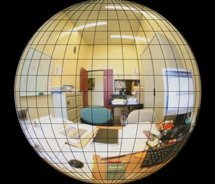
Load the spherical representation of your scenary and run the command:
>GRID SPHERE 0
The first parameter is the designation of the actuel projection (here a spherical projection because the first value of the description file is 0). The second parameter is the intensity of the drawed coordinate grid. The result:
Now, edit the ASCII file
0
0 140 0
848 727
424
364 370
0 0
-180 180 -90 90
0 0
0 1
10 10 3
and save under the name SHERE2.LST. The only difference with the SHPERE.LST is the value of the north pole latitude (140°, not 90°). Run the MAP command:
>MAP SPHERE SPHERE2
The syntax is very simple. The first parameter is the name of file description of the actual projection. The second parameter is the name of file description of the destination projection. Here, the new projection is a very similar spherical projection, but now, the pole is tilted by a angle of 140°-90°=50°. You can also draw a coordinates grid on the new generated image:
>GRID SPHERE2 1500
The result:
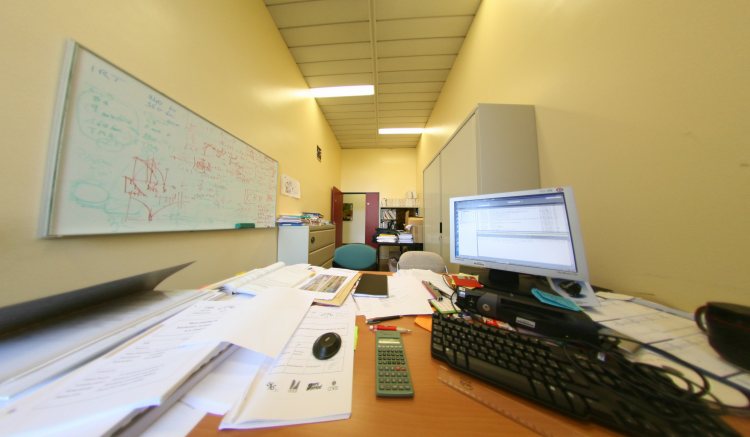
The
tilted sphere.
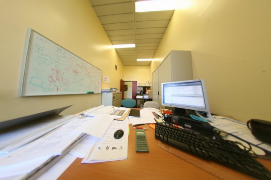
The pocket calculator is now nearly face on (the contour is not strictly rectangular because the calculator is not at an infinity distance, so some perspective distorsion are present).
Edit a new description file, and save with the name CYLIND.LST:
1
0 0 0
0 0
0 0 0
0
0
-90 90 -60 60
0 0
0 0.2
10 10 3
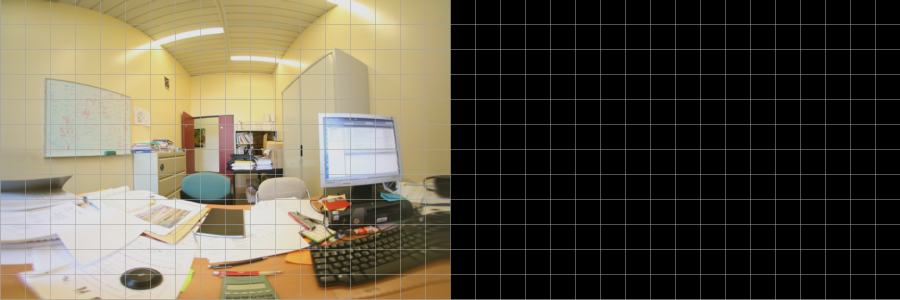
It is the description of a simple cylindric projection (panoramic projection). Reload the starting spherical projection image, then
>MAP SPHERE CYLIND
>GRID CYLIND 2000

The
image cover an angular range of -90, 90° along horizontal direction and
+/-60°
along the vertical direction (see the CYLIND.LST file content) .
It is very easy to reverse the process (after modification or not of the cylindar projection image):
>MAP CYLIND SPHERE
It is easy to synthesize 360° panorama, by combining two of more fisheye images. Modify the CYLIND.LST file to a CYLIND2.LST file:
1
0 0 0
0 0
0 0 0
0
0
-180 180 -60 60
0 0
0 0.2
10 10 3
Note the new output longitude range is of (-180°, +180°).
Modify also the input spherical projection (save the modification with the SPHERE3.LST):
0
0 90 90
848 727
424
364 370
0 0
-180 180 -90 90
0 0
0 1
10 10 3
The central meridian is shifted by an angle of 90° (parameter #4). Run
>MAP SPHERE3 CYLIND2
>GRID CYLIND2
2000
The
actual image cover the left part of a future 360° mosaic.
Compute now a sinusoidal projection starting from the 360° cylindrical projection. Create the SINUS.LST file:
5
0 0 0
0 0
0 0 0
0
0
-180 180 -70 70
0 0
0 0.2
10 10 3
>MAP SPHERE SINUS
>GRID SINUS 2000
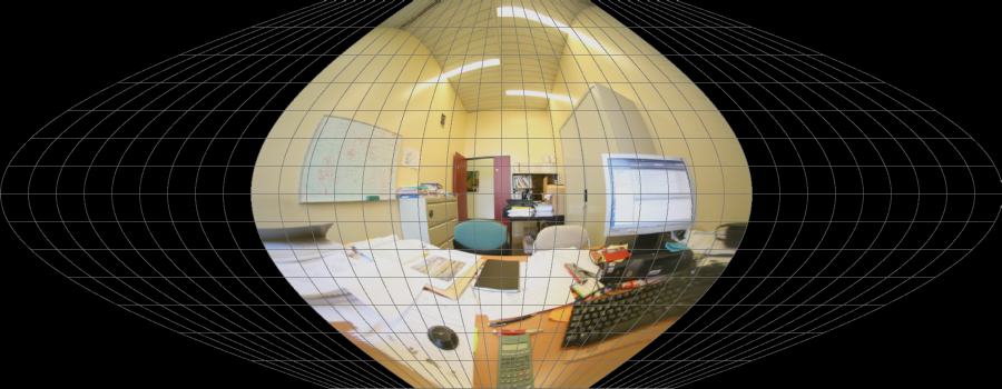
The
180° image on a 360° sinusoidal projection. Note the minimal distorsion along the
central meridian (a characteristic of the sinusoidal projection).
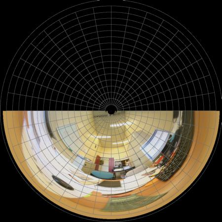
A last example, a polar projection. Save the POLAR.LST file with the content:
7
0 0 0
0 0
0 0 0
0
0
-180 180 -90 90
0 0
0 0.4
10 10 3
then
>MAP SPHERE POLAR
Nearly 300 projections combinations are
possibles! You can also create spectacular animation (rotation around a point
of view for example), etc. Here some demonstration
examples.
Correcting the optical distortion
Consider the following image taken with a Canon EOS 5D and a Canon zoom USM 17-40 mm used at 17 mm:
Example
of noticeable barrel distortion.
For correct these distortions Iris perform a shifting of each pixel radially. The computed function is a third order polynomial. The coefficients of the function (A, B, C, D) are specific to a given lens, and can be reused for each image taken with this lens. The form of the radial fitted function is:

The parameter D adjust the scale of the final image. If A=B=C=0 and D=1, the image is not modified. Negative values are of course accepted, for correct pincussion distortion. You can merge positive and negative values. For example, a negative value for the A coefficient can correct pincussion distortion of the outmost pixels.
For a first step, the coefficients can be evaluated interactively. Run the Distortion adjustment... command of Geometry menu, then
The parameters are: A=0, B=0.028.10-6, C=0.210.10-3, D=0.93. For a first evaluation you can use a a tiny version of the original image. For a fast calculation, Iris use also here a simple bilinear interpolation.
For the final correction, open the dialog box Correct distortion... of Geometry menu and select the Bicubic option for a high-quality sampling method with negligible image degradation:
If necessary, crop the useful part of the corrected image: You can also insert a grid in the image for help to check the result (Frame... command of View menu):
The
processed image.
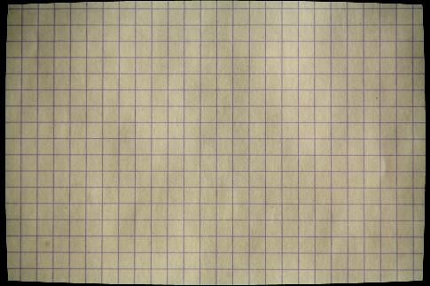
The polynomial coefficients can be found from points measured in a photography of a regular grid. For example, here a grid seen through an objective lens Canon 24-70 mm (macro position):
With the assistance of the mouse pointer, measure the position of pixels corresponding to the intersection of the grid, for example along an horizontal axis. Start from the center of the image:
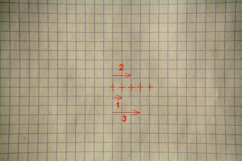
Write a text file with columns. The first contains the coordinates raised in the image. The second corresponds to the coordinates find if the optics presented not distortion. The unit in this last column does not have importance. Here one selected a regular step with an increment of one unit. This gives the contents of following file:
0 0
167 1
331 2
498 3
664
4
830 5
995 6
1168 7
1334 8
1506 9
1678 10
1856 11
2033
12
Save the file in the working directory with the name grid.dat (only the extension is imposed).
Since the console, run the command FITDISTOR with the parameters::
>FITDISTOR grid 4
The first parameter is the name of the text file containing the coordinates measured in the image. The second parameter is the degree of the polynomial which is adjusted through the measured points. Here the result in our example:
RMS is the quadratic error of the fit of the second column of the file. More the error value is small, better is the adjustment. Run the command Distortion correction... of Geometry menu:
All the automatically filled. Click OK for process the image. Here the result:
Note that for the majority of the situations, a second order polynomial is sufficient (see the small value of the 4th degree coefficient in your example).
Tip 1: The command FIT is a general function for fit a polynomial function on the data saved in a text file (two columns format). For example:
>FIT GRID 6
An O-C file is created automatically in the working directory (OC.LST)
Tip 2: You can process the R, G and B channel
individually for correct lateral chromatism aberration for example. Split the
48 bits image (SPLIT_RGB command), adjust distortion of each channel and recombine
the color image (TRICHRO command).
Correcting perspective
Load an image and run the Perspective adjustment... command of Geometry menu:
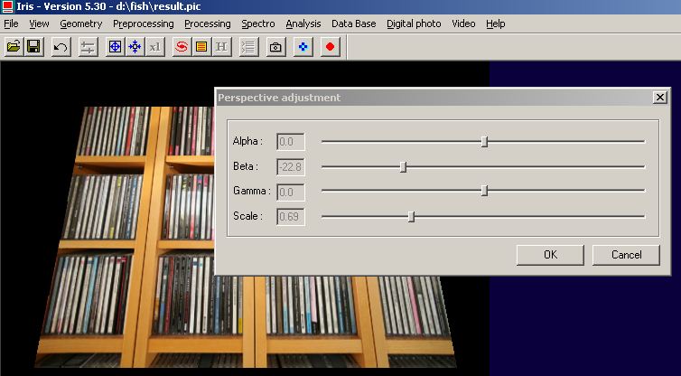
Interactive
selection of the perspective.
Here some typical perspective effect, function of the selected angle:
|
|
|
|
|
|
For the final processing run the command Perspective correction.... of Geometry menu and select Bicubic sampling option. You can also define the size of the final image:
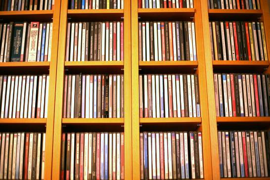
The
perspective default to correct...
...and
the image after perspective processing.
The optical distortion can be corrected first (see the
following paragraph).
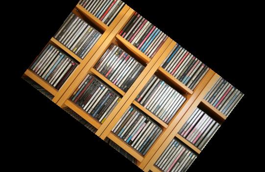
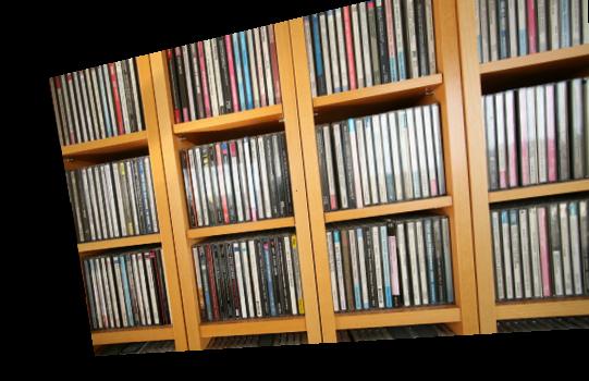
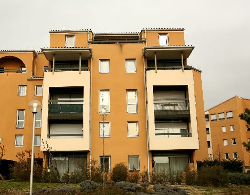
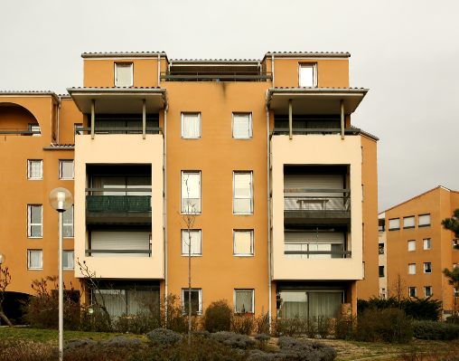
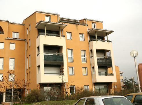
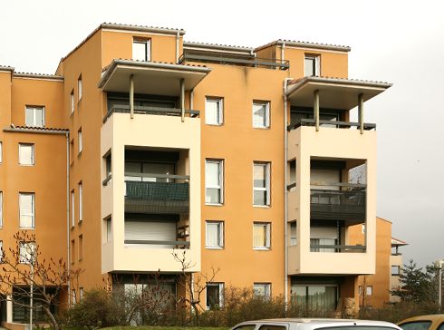
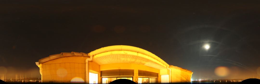
Here another traditional example, on an image of a building:
|
|
|
After the use of the perspective tool, the image above has undergoes a very final and slightly improvement by scaling the vertical axis. The goal was to maintain a circular contour for the first plane lamp. The operation is easy by using the Resample tool... of Geometry menu. The scale factor applied along the horizontal axis is 1 (no modification) and 0,96 along the vertical axis:
Note: The Bicubic interpolation is recommended for non-astronomical images, but, for deep-sky images, the Spline method is preferable because the natural aspect of stars is more preserved.
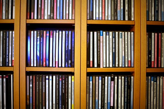
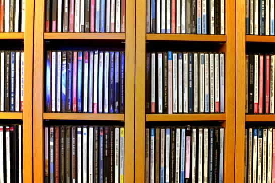
The last example is more problematic because multiple angles are concerned. The parameters are easily to find by using the interactive perspective tool. The degree of correction is in any case enough subjective, strongly related to the appreciation of the operator and the destination of the image:
|
|
|
Correcting the vigneting default
The console base command is CVIGNE2. Syntax:
CVIGNE2 [IMAGE] [TEST]
[IMAGE] is the name of the image file to correct. [FLAT] is the file name of an uniform screen taken in the same conditions (same lens, same aperture). Iris adjust a second order polynomial function onto the "flat" image and applied the inverse polynonial function to the image to be corrected. The result is displayed on the screen after processing. Example:
Image of a white screen. The image is acquired with a
Canon lens 50mm @ f/1.4 and a EOS 5D..
The optical vigneting is clearly visible (obscuration on the edges).
The image is saved with the name FLAT (for example).
|
|
|
The alternative method is to use the EVIGN and CVIGN commands.
EVIGN
Load the "flat" image and run the EVIGN command (no parameters). Iris return the polynomial coefficients in the output window:
Relative to the X distance from the image center, the vigneting is modeled by the function:

CVIGN [A] [B] [C]
Apply the vigneting correction with the given polynomial coefficients. Load the image to correct, then
>CVIGN -1.125e-7 -2.654e-5 1.153
|