New features of version 3.83(b) (August 26, 2003)

Revision 3.83b (August 26 2003) - Addition of processing function of the edge of planets, optimization of certain functions for colors image processing.

Revision 3.83a (August 17 2003) - New functions loading Digital Camera images (tested with Canon D60 / 10D / 100D, Nikon D100, Canon Powershot G3, Minolta DiMAGE7, Nikon CoolPix 950/990/995).

Attenuation of the effects edge during the planetary image processing

To visualize the details contained in a planet image the fuzzy mask and the wavelets (multi-scales processing) are effective tools. But bright can appear around the planetary disk:

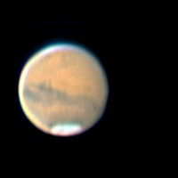
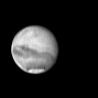
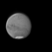
For this example the image of Mars is taken on August 3 2003 by Marc Rieugnié (Saint-Caprais) with a 400-mm telescope, a Barlow 2x and a webcam ToUcam Pro. On left, there is the rough image resulting from the addition after register of 150 frames selected on a total of 600. At right, the image was processed rather vigorously by the wavelet technique for better seeing of the details. But, one notes the appearance of an arc edging on the left side of planet. It does not have physical reality, it comes from the processing applied. It is an artifact. The fact that it is present on the left edge of planet and not on the right edge is due to the phase effect of phase at the time of the observation. The left edge is more abrupt than the right edge and this small difference is enough to explain the behaviour of the processing. Also, the problem is accentuated by the presence on the left (especially in top of the image) of real bleue clouds into the Mars atmosphere.

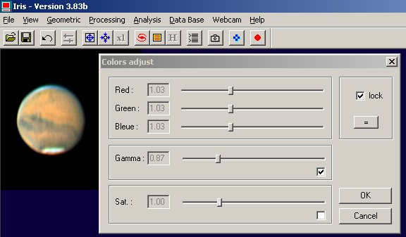
The version 3.83b add a tool for correct this problem. Display the tri-color image, for example enter the command TRICHRO R G B since the console, with R, G and B are names of the files respectively containing the layers red, green and blue of the color image. Run the Wavelet... dialog box from Processing menu:

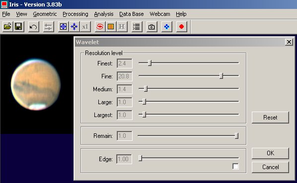
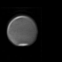
The version 3.83b adds a little more interactivity compared to the preceding versions. The function making it possible to reduce the effects effect is accessible at the bottom of the dialog box. Check Edge option and move the slider.

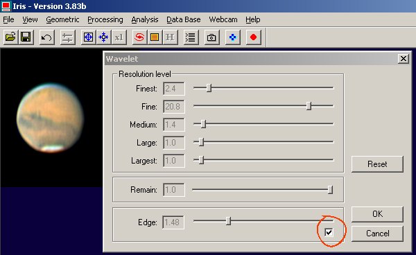
Use this adjustment with much parsimony! To note for example that we preserved the fogs polar blue haze here. To validate click the OK button.

The dialog box Unsharp masking... (Processing menu) profits from the same improvements (processing of the edge of planets and direct work on the images colors):

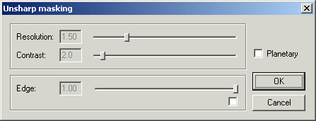
Note: the new command UNSHARP3 as similar effect has the new unsharp masking dialog box..

You can refine with final the balance of the white with corresponding dialog box of visualization menu. The calculations carried out by this function were accelerated of a factor 3 in the version 3.83b compared to the former versions.

The result can be saved in the form of 24-bits BMP image 24 bits. For example: SAVEBMP RESULT

The version 3.83b add significant function for the management of the images colors: SAVE_TRICHRO (or SAVE_TR in compact form). It save in three files the three colors layers displayed in the current image. For example:

SAVE_TR R2 G2 B2

SAVE_TRICHRO is symmetrical that TRICHRO (TR for a compact form) which uses three black&white image to display a true colors images onto the screen.

Here the aspect of the three black&white images after SAVE_TRICHRO command, respectively the red, green and blue layers (a new color visualization is always possible by typing  TR R2 G2 B2):

The new COMPOSIT2 command
and... a summary of the stacking methods under IRIS

ADD2 [NAME] [NUMBER]
The output image is the simple sum of the input images of generic name [name] (ex. M57-1, M57-2, M57-3...). The number of image added is [number]. The final value do not exceed 32767, i.e. a pixel value after the sum is truncated to 32767 if this the sum is superior to 32767. The use of the very similar command ADD_NORM scale the input value of the pixels for normalize the max intensity of the final image to 32767 (after the stack).

SMEDIAN [NAME] [NUMBER]
The output image is the median of the input images at each pixel (generic name [name]). The median of the [number] images is the ([number]+1)/2 th value of the sorted pixel values at each point in the images. This is the average of the two middle values for an even number of images. The SMEDIAN command use a relatively fast algorithms and this command is a good choice if there are a low number os images (<19). For more than 19 input images use the command SMEDIAN2 (same syntax).

COMPOSIT [NAME] [COEF. SIGMA] [# ITER] [FLAG MAX] [NUMBER]
Input images are stacked by applying a sigma-clipping algorithm at each pixel. Compared to median technique, sigma-clipping only rejects the most highly deviant values, so the result includes more of the data and so  in most case the signal to noise is increased. COMPOSIT works best when many images are available (more than 10 ideally). The input number of image is virtually unlimited (it is a new important improvement of the version 3.83). For a given pixel, after a mean is computed, one computes a deviation of the pixel from the mean and then compares it with a the clipping-sigma rejection criteria. If the deviation exceeds [coef. sigma] times the local RMS noise, then the pixel under test is regarded as being bad. After the bad pixel is rejected, one iterates the process, but now the mean and the noise are re-calculated, excluding the bad pixels already rejected in the previous iterations. The number of iteration is given by the parameter [# ITER]. Typical value for parameters are [coef. sigma]=3 or 4 and [# iter]=2. Successive test are necessary for determine the optimal parameter value for reject cosmic rays and bad pixels. To avoid removing real data do not use a value of [coef. sigma]<1.5 (too value rejected, i.e. the signal to noise ratio significantly decrease). After the deviant pixels are rejected the final add is computed from the remaining data. If [flag_max]=0 a simple sum is computed, if [flag_max]=1 input images are scaled and the upped value of the final stacked image is normalized to 32767 (same procedure as ADD_NORM).

COMPOSIT2 [NAME] [FLAG. MAX] [NUMBER]
COMPOSIT2 method use a robust average image using a continuous adaptive weighting scheme that is derived from the data themselves -  see Artificial Skepticism Stacking algorithm  - Stetson 1989, V Advanced School of Astrophysics [Univerisidade de Sao Paulo], p.1. See also: http://archive.stsci.edu/hst/wfpc2/pipeline.html
http://archive.eso.org/archive/hst/wfpc2_asn/3sites/WFPC2_Newsletter.pdf

The given parameters are only the generic name of the input image sequence, the normalized flag (0 or 1, see COMPOSIT) and the number of input image (an unlimited number).

The weights of the pixel values are computed by the equation:

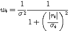
where w_i is the weight of the i ^th pixel value, s_i is the sigma of the i ^th pixel in the stack, derived from the readout noise and camera gain. The r_i term, which is the residual between the current average pixel value and the value of the i ^th pixel, is computed at each iteration. This version of COMPOSIT2 use classical and internally coded value for CCD readout noise and camera gain (noise of 15 electrons RMS en 2 e-/ADU). COMPOSIT2 is a simple command to use and efficient for bad pixels rejection.

Important, before use commands like SMEDIAN, COMPOSIT and COMPOSIT2 it is necessary to have the same sky background level for all the images of the sequence. Use the command NOFFSET if is not the case (or NOFFSET2 for select a specific region for the harmonization of the sky level). Similar, is the exposure time is not the same the image should be scaled before stacking (MULT, MULT2, NGAIN2 commands for exemple).

The choice of the most optimal combining algorithm will depend on the nature of the data and on the exposure type. For produce a clean flat-field or a master dark frame the appropriate command is SMEDIAN (or SMEDIAN2). For deep-sky imaging the classical sigma-clipping is a good choise for the best conservation of signal to noise (the median lose 30% in signal to noise typically relative to simple sum and the COMPOSIT/COMPOSIT2 commands). The COMPOSIT2 command  is now an useful and fast altenative to the sigma-clipping scheme.

L_OPTBIN and L_OPTBIN2 : Optimal extraction for CCD spectroscopy

We implement in this version of IRIS algorithms to reduce with high quality two-dimensional spectra into one-dimensionnal spectra. The very standard technique is to sum the columns (spatial direction, i.e.  perpendicular of dispersion axis) which include significants amounts of starlight. The operation is done after sky subtraction (see L_SKY family commands). The Iris commands for this sum are for example L_ADD (manual entry of limit of the spectrum along columns) or L_BIN (automatic determination of the spectrum extend along columns).

The optimal extraction method consist to assign to each pixel, when the summation takes place, a weighting factor proportional to the amount of the signal in it. We have implemented two algorithms for this, described in two classical paper:

J. C. Robertson, PASP, 98, 1220-1231, November 1986 - Coded and adapted in the command L_OPTBIN
K. Horne, PASP, 98, 609-617 - June 1986, Coded and adapted in the command L_OPTBIN2

The Robertson's algorithm (L_OPTBIN command) is applicable only when the detector columns are perfectly aligned perpendicular to the dispersion direction. If it is not the case at the acquisition time, a post-operation consist for example to apply the TILT command. Although L_OPTBIN is still useful because it is robust and fast method, and yields good results if such a small misalignment is present.

The Horne's algorithm (L_OPTBIN2 command) is very time consuming (fit of many low-order polynomials along the spectrum). It work for tilted or distorded spectra. But, attention, this algorithm cannot be used if variation in the fraction of starlight falling onto pixels have a more complex form than can be fitted with low-order polynomials. So generally, we prefer use the Robertson algorithm and manual geometric correction of the spectrum  (command SLANT, TILT, SMILE, ...).

For this two commands it is necessary to give estimation of the mean sky level in ADU (Analog Digital Unit, or Counts). But, very important, before application of L_OPTBIN or L_OPTBIN2, the sky is removed of the processed image (use L_SKY, L_SKY2, L_SKY3). The following parameters are the electronic gain of the camera in electrons/ADU and the readout noise (RON) of the CCD camera in electrons. A final parameter (kappa), is a coefficient for adjust cosmic (or hot spot) rejection process (similar to the kappa parameter in the kappa-sigma rejection method (or sigma clipping) for staking images - see COMPOSIT or COMPOSIT2 commands).

The syntax are:

L_OPTBIN [LINE1] [LINE2] [GAIN (e/ADU)] [RON (e-)] [MEAN SKY LEVEL (ADU)] [KAPPA]
L_OPTBIN2 [LINE1] [LINE2] [GAIN (e/ADU)] [RON (e-)] [MEAN SKY LEVEL (ADU)] [KAPPA] 

LINE1 and LINE2 are the lines coordinates upper and lower the star spectrum. Thanks to the optimal extraction it is possible to select a relative wide range between LINE1 and LINE2 for an optimal photometry (summation of 10 to 20 lines for example is classical).

Here, some exemples...

TEST IMAGE 1: Spectrum of the B9V type star HD172671 (V=6.1). It is a single 180-s exposure with the MERIS spectrograph linked to the telescope (a 128-mm Takahashi refractor) by a 100-microns optic fiber. Click here for a full description of the setup. The camera is an Audine KAF-0401E model, used at bin 2x2. The gain of the Audine is 2 electron/ADU. The detector noise is estimated to 25 electrons (RON + some thermal signal). The mean spectral sampling is of 5.74 A/pixel.

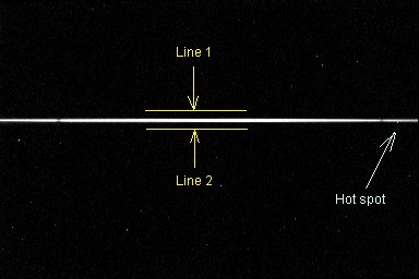
The background sky level is very low, we take 0. By definition the signal level outside the star spectrum is zero in a fiber spectrograph. The TILT command is used to align precisely dispersion along CCD lines. The graphs below show the 1D spectrum for respectively a standard sum between the CCD line 138 and 155 (a too wide range) i.e L_ADD 135 155, an automatic selection of lines position for bin 98% of the starlight signal (the Iris L_BIN command select the lines 144 and 148), and an optimized extraction with the command:

L_OPTBIN 155 138 2 25 0 15

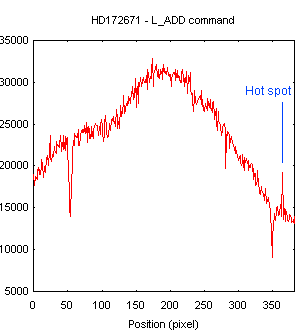
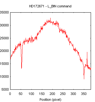
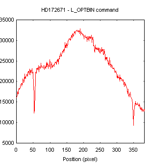
For this example, compared to L_BIN procedure, the optimal extractive scheme increase the signal to noise ratio by a factor 1.16, and consequently the effective exposure time by factor 1.34 (square of 1.16). It is a very significant gain ! Note also the elimination of the hot-spot. For the good value for kappa parameter is estimated by successive try. Values of kappa parameter between 5 and 50 are typical (15 for this exemple). More precisely, to select the value of kappa, survey the information on the number of excluded pixels returned by the command L_OPTBIN (or L_OPTBIN2). A good value is for a keep pixel number oscillates between 0 and 1 For turn-off rejection procedure of L_OPTBIN command, for example because no cosmetic default are presents in the spectrum, adopt a large value for kappa, for example 100.

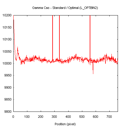
TEST IMAGE 2: Spectrum of the star Gamma Cas (Be-type) (MERIS spectrographe + Takahashi FS-128 refractor). The signal to noise is here very high. But the example is difficult : (1) the spectrum is undersampled, (2) we hope remove cosmic rays (artificial for this simulation) but not the true spectral emission lines !

The result of L_BIN and L_OPTBIN 80 55 2 12 50 40:

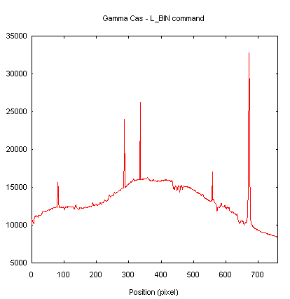
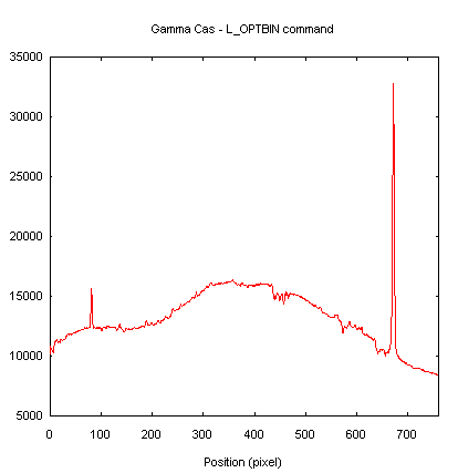
The detectivity  gain is not significant in this high signal to noise case, but the pixel rejection scheme is successful.

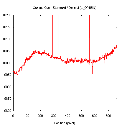
The next figure present the ratio of the standard and optimal result normalized to 10000. The standard and the optimal extractions are identical at 1% photometric precision. It is a good result. The limitation is the variation of the spectrum wide along the dispersion axis (chromatic aberrations effect of the dioptric optic used in the spectrograph). For an ultimate photometric precision an improvement consist to process only part of the spectrum at the same time. We can see also the result with the L_OPTBIN2 command (Horne scheme): the spectra are nearly indistinguishable at a level largely better than 1% (expect at the border for polynomial fit problem reasons). The large glitches visible in the ratio are the cosmic ray detected an rejected by the optimal extraction algorithms..

TEST IMAGE 3: Spectrum of the star 4 Aql (Be-type) acquired with the 24-inch telescope of Pic de Chateau Renard (AstroQueyras + team of Lyon-Ampère association). The effective resolution of the spectrograph is of 11000. The starlight is distributed on the CCD surface through à set of fiber bundle. 300-seconds exposure with a ST8E CCD camera (readout noise of 12 electrons RMS).

The next figure show spectra of 4 Aql extracted with standard procedure (L_ADD 87 131) and optimal procedure (L_OPTBIN 87 131 2 12 0 5):

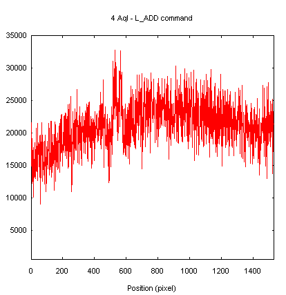
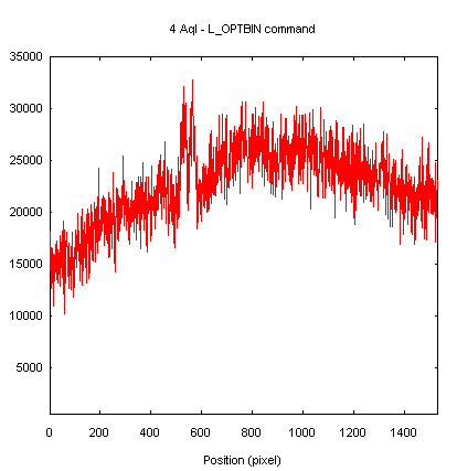
The increased signal to noise ratio obtained with the optimal extraction procedure is very evident

OTHER NEW COMMANDS

ADD_NORM2 [ NAME ] [NUMBER]
Same command that ADD_NORM (addition of a sequence of images and normalize the most intense pixel to 32767 if necessary), but the zone where normalize is computed is selected with the mouse. This gives flexibility for some situation cases to avoid saturating a specified part of the image.

REINDEX [IN] [OUT] [FIRST INDEX IN] [FIRST INDEX OUT] [NUMBER]
Reorganize the indices of a sequence. Let us suppose a sequence: I1, I2, I3, I4. One wants to transform it into a sequence J5, J6, J7, J8. One will write:

REINDEX I J 1 5 4

The input and the output sequences cannot have the same name. [number] is the number of image to be converted.

SAVE_TRICHRO [R] [G] [B] (or SAVE_TR [R] [G] [B])
Save the colors layers of the current displayed true color image into three distinct file.

TRANS2 [ IN] [OUT] [DX (PIX./HOUR) ] [ DY (PIX./HOUR) ] [NUMBER]
Transform a sequence of image into another sequence by making a translation of a certain number of pixels depending on the hour of acquisition of the images and the shift in X and Y specified in parameters (in pixels per hour). The typical use is the centering of a sequence on the movement of a comet or of an asteroid in such a way that this object appears fixed after stacking. One generally proceeds in two times: registration on a star of the field (REGISTER command for example), then, application of the command TRANS2 command. Supposing that the ephemeris (or a direct measurement in the image) teach us that mobile object moves 0.230 pixel/hour in X and of -0.763 pixel / hour in Y in the sequence I1, I2, I3... I20. One obtains a new sequence J1, J2.... J20 where the movement of the object is cancelled while making:

TRANS2 I J 0.230 -0.763 20

Click here for an exemple of the use of TRANS2.

BLACK and WHITE commands

To restore just colors of tri-color images it is some time necessary to the balance the white. The version 3.83b integrates two new commands which make it possible to carry out this operation with precision and speed. The first is the function BLACK which bring the sky background to zero in a zone selected with the mouse, and that simultaneously on the 3 colors plans in memory. For example, define a rectangle in part of the image where the sky is naturally black, like this:

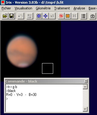
The command return the background levels of sky in the zone for the three plans. These levels are automatically subtracted and the result is displayed.

The second command, WHITE, makes the adjustment of the white itself. The three colors planes are treated simultaneously (as opposed to what made SCALECOLOR2 command). One selects a reputed white area in the image with the mouse (Iris calculates the median intensity in the window). In the case of the planet Mars the polar cap is ideal for that (but attention, one should not have saturated the image at this place due for example to a too long exposure time). Here the example:

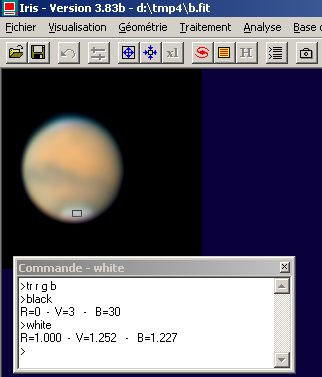
Iris turns return the coefficients by which it has to multiply components RGB to adjust the levels in the selected zone. Note that commands BLACK and WHITE must be executed in the order given hereafter.

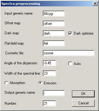
The possibility of entering manually a tilt angle was added in dialog box Spectra preprocessing. The tilt angle is the angle between the dispersion axis and the CCD lines. The possibility of an automatic correction of the tilt of the old versions (and also of the possible curve) was preserved (check the Auto. button).